
A historical test produces excellent results. Then the model is used before real matches and the improvement disappears.
There are several possible explanations: changed conditions, too little data or a model chosen to fit the test period. One deserves checking early because it is so easy to miss: the historical test may have known things that the live forecast could not know.
In football, the database makes this particularly tempting. It holds the fixture, the outcome and the finished match's statistics together. A convenient join can turn tomorrow's information into an apparently ordinary input column.
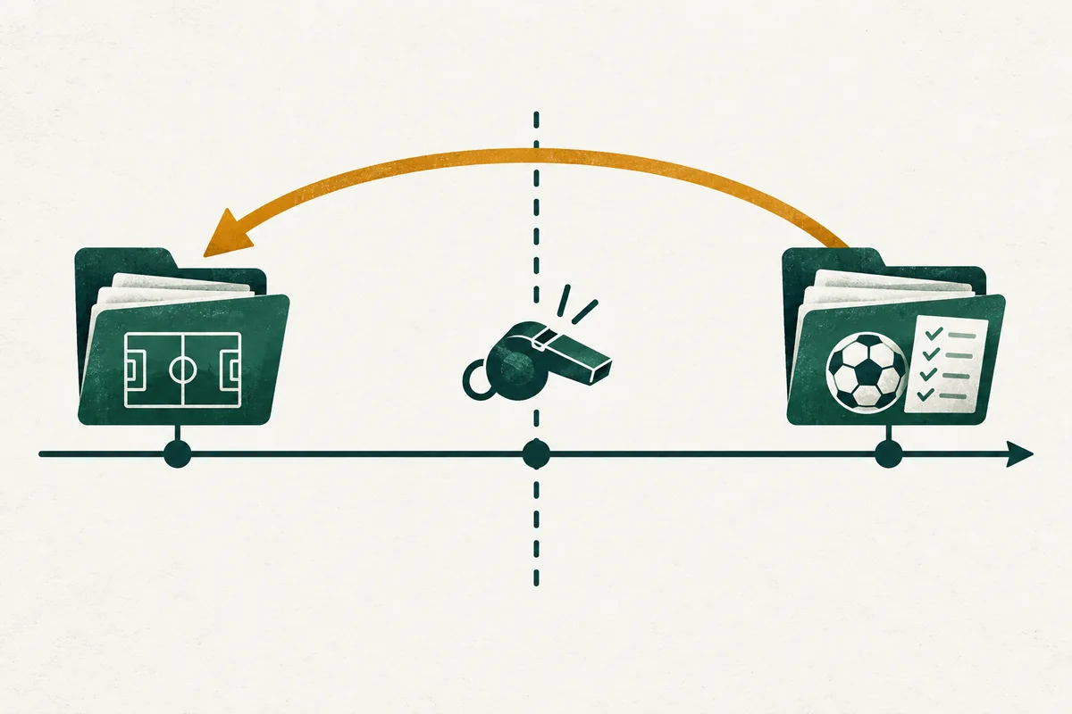
The cutoff is part of the forecast
Consider a hypothetical timeline for a Saturday fixture:
| Time | Available information |
|---|---|
| Friday, 18:00 | Preview published; earlier results and available team news can be used. |
| Saturday, 14:00 | Official starting lineups become available. |
| Saturday, 15:00 | Match kicks off. |
| Saturday, 17:00 | Result is known; match statistics may still be incomplete. |
| Sunday, 10:00 | Provider revises or fills some statistics. |
A Friday-evening forecast cannot use Saturday's starting lineup merely because the lineup now appears on the fixture page. A forecast twenty minutes before kickoff can use it if it was actually available then. Neither can use the match's eventual xG as a pre-match feature.
The precise times here are illustrative, not claims about any competition's announcement schedule. The rule is about availability, not one standard hour.
Event time and availability time are different
A statistic can describe a match played yesterday but only reach the system this morning. Its event time is yesterday; its availability time is this morning.
A backtest filtering only on match dates may use it for a forecast supposedly produced last night. That is still leakage, even though the event happened before the forecast.
For repeatable evaluation, preserve when an observation became usable and which version was used. A later provider correction should not silently overwrite the historical inputs used to judge the model.
If availability history was never recorded, acknowledge the limitation. A reconstructed historical test can still be useful, but it should not be described as an exact replay of live decision-making.
The rolling window can include the target
A "last five matches" feature is a frequent culprit. Build it on a season table that already contains the target match and it may include the result you are trying to predict.
For a simple sequence of completed fixtures for one team, the conceptual operation is:
feature for fixture t = aggregate of eligible observations before t
A shifted rolling calculation can enforce that exclusion in a clean, correctly ordered sequence. It is not a complete solution for football data. Postponements, simultaneous fixtures, team identifiers, competition boundaries and late-arriving metrics all need handling.
Check a handful of rows manually. For each target match, print the identifiers of the observations used to build the feature. A feature name such as pre_match_form is not evidence that the implementation respected its cutoff.
A chronological split helps, but does not repair future features
Training on earlier periods and evaluating on later periods better resembles live use than randomly mixing a season's fixtures. Still, splitting by time does not make a leaked column safe. A feature containing the final league position or current full-season averages may already include later results.
There is also leakage from preprocessing. If scaling, imputation or feature selection is learned from the entire dataset before the split, the evaluation period influences the model-building process. Fit those steps on the training data and apply the learned transformation to held-out data.
The scikit-learn pitfalls guide documents this issue. Its TimeSeriesSplit reference is useful too, but notes an equal-spacing assumption for comparable fold durations. Football fixtures are irregularly scheduled; date-based blocks may be more appropriate than blindly using the default row-based splits.
Tuning can turn the test set into training data
Suppose a researcher tests twenty rolling windows, five league filters and several confidence thresholds, then publishes the combination with the best result. No final-score column has leaked, but the supposedly held-out period has still guided method selection.
Use a validation period for those decisions and reserve a later test period for the final evaluation. If the method is changed after looking at the final test, call the new result exploratory and arrange another test.
A small improvement should also be compared with a fixed baseline on the same fixtures. Better Brier scores or calibration plots cannot compensate for contaminated evaluation inputs.
A practical audit before trusting the headline
Ask the researcher to show one target fixture with its original input snapshot. Trace each feature to a source observation and an availability time. Confirm that no target-match statistics or later revision entered the input.
Then check the split: what was trained, what was tuned, and what remained untouched until the final evaluation? Inspect how missing values were handled; a current backfill can erase a missing-data situation that the live system really faced.
Finally, look for a live or forward-recorded sample. A smaller sample recorded prospectively may offer stronger evidence about the published process than a much larger retrospective test with uncertain data provenance.
XG Mind's methodology page and public record should be examined under the same standard. This article describes an audit procedure, not a claim that an independent audit has certified every part of the platform.
The shortest useful question is: could the system really have known this value then?
Sources: Scikit-learn: common pitfalls and data leakage; TimeSeriesSplit documentation. The match timeline is a constructed example.